Объединение риска
Материал из Supply Chain Management Encyclopedia
Storch (обсуждение | вклад) |
Storch (обсуждение | вклад) |
||
| Строка 14: | Строка 14: | ||
Чем выше корреляция между риском различных объектов, тем меньше разница между ''риском от объединения'' и ''необъединенным риском''.<ref>Simchi-Levi, D., P. Kaminsky and E. Simchi-Levi (2000), ''Designing and Managing the Supply Chain'', Irwin Mc-Graw Hill, Boston, p.56-60.</ref>. Фундаментальной выгодой от объединения риска в управлении цепями поставко является то, что более низкий риск можно условно приравнять с более низкой вариацией, а более низкая вариация в системе управления поставками обычно означает меньший уровень страхового запаса. Посредством более низкого страхового запаса объединение риска может понизить стоимость поддержания запасов без снижения уровня обслуживания. В итоге для принятия решения нам нужно выбрать между выгодами объединения риска (то есть более низкий страховой запаса) и затратами на реализацию стратегии объединения риска. | Чем выше корреляция между риском различных объектов, тем меньше разница между ''риском от объединения'' и ''необъединенным риском''.<ref>Simchi-Levi, D., P. Kaminsky and E. Simchi-Levi (2000), ''Designing and Managing the Supply Chain'', Irwin Mc-Graw Hill, Boston, p.56-60.</ref>. Фундаментальной выгодой от объединения риска в управлении цепями поставко является то, что более низкий риск можно условно приравнять с более низкой вариацией, а более низкая вариация в системе управления поставками обычно означает меньший уровень страхового запаса. Посредством более низкого страхового запаса объединение риска может понизить стоимость поддержания запасов без снижения уровня обслуживания. В итоге для принятия решения нам нужно выбрать между выгодами объединения риска (то есть более низкий страховой запаса) и затратами на реализацию стратегии объединения риска. | ||
| - | == | + | ==Пример: Объединение риска по продуктам== |
| + | |||
| + | Хорошо известный пример компании Dell, которая отложила сборку компьютеров до того момента, когда появлялся точный заказ от конечного потребителя, иллюстрирует концепцию сборки на заказ. Компоненты компьютеров готовы к сборке, однако окончательная конфигурация продукта откладывается до того момента, когда поступит заказ от потребителя. Компания HP иллюстрируют | ||
The well known Dell example of delayed assembly until after orders arrive well illustrates the concept of assemble-to-order. Component parts are ready for assembly, however, the final configuration of the product is delayed (or postponed) until after orders have arrived. HP illustrates the strategy of form speculation: products are made-to-stock based on forecasting (see [[order penetration point]]). Supposed a company manufacturers two products, SKU 4501 and 4502. The production [[lead time]] for each product is 21 days and we shall assume for expository purposes that the lead times are constant. As seen in Table 1, respective average weekly demand for the SKUs are 1200 and 2200 and respective standard deviations in weekly demand are 170 and 230. Using the [[inventory model with uncertainty in demand and lead time]] provides respective average safety stock levels of 1,597 amd 2,161, for a total average safety stock level of 3,758. | The well known Dell example of delayed assembly until after orders arrive well illustrates the concept of assemble-to-order. Component parts are ready for assembly, however, the final configuration of the product is delayed (or postponed) until after orders have arrived. HP illustrates the strategy of form speculation: products are made-to-stock based on forecasting (see [[order penetration point]]). Supposed a company manufacturers two products, SKU 4501 and 4502. The production [[lead time]] for each product is 21 days and we shall assume for expository purposes that the lead times are constant. As seen in Table 1, respective average weekly demand for the SKUs are 1200 and 2200 and respective standard deviations in weekly demand are 170 and 230. Using the [[inventory model with uncertainty in demand and lead time]] provides respective average safety stock levels of 1,597 amd 2,161, for a total average safety stock level of 3,758. | ||
Версия 23:42, 16 августа 2011
English: Risk pooling
Объединение риска предполагает процесс агрегирования объектов в группу, чтобы уровень риска для всей группы оказался меньше суммы рисков для индивидуальных объектов. Математически это может быть выражено следующим образом:

Где:
- Oi = объект i.
Одной из основных областей применения объединения риска является страхование. Однако, оно применяется также в различных других областях, включая экономическую теорию и управление цепями поставок. В экономической теории вертикальная интеграция (См. Аутсорсинг) менее вероятна в том случае, если фирмы формирует "небольшую часть общего спроса на ресурс, поскольку в данном случае они потеряют экономию от объединения рисков на большом рынке после интеграции. Стимулы для интеграции могут увеличиваться, если спрос со стороны других фирм на ресурсы крайне изменчив, создавая таким образом условия для повышения цены".[1]. В управлении цепями поставок существует два основных применения объединения риска: отсрочка формирования (form postponement) и географическая отсрочка (geographic postponement). В первом случае агрегированные объекты представляют собой продукты (то есть объединяется риск по различным продуктам), и его противоположная стратегия называется спекуляцией формирования (form speculation). При отсрочке формирования производство конечной формы продукта откладывается до того момента, пока получен заказ (см. Точка проникновения заказа). В географической отсрочке агрегируемые объекты представляют собой географические регионы (то есть осуществляется объединение риска в пространстве), а его противоположность называется географическая спекуляция (geographic speculation). При географической отсрочке используется меньшее количество складов. Таким образом, фирма откладывает принятие решения о том, где необходимо разместить запасы до того, как будет получен заказ.
Если риск объектов независим, тогда более высокий риск одного объекта будет компенсировать низкий риск другого. Если происходит, тогда объединенный риск < необъединенного риска Чем выше корреляция между риском различных объектов, тем меньше разница между риском от объединения и необъединенным риском.[2]. Фундаментальной выгодой от объединения риска в управлении цепями поставко является то, что более низкий риск можно условно приравнять с более низкой вариацией, а более низкая вариация в системе управления поставками обычно означает меньший уровень страхового запаса. Посредством более низкого страхового запаса объединение риска может понизить стоимость поддержания запасов без снижения уровня обслуживания. В итоге для принятия решения нам нужно выбрать между выгодами объединения риска (то есть более низкий страховой запаса) и затратами на реализацию стратегии объединения риска.
Пример: Объединение риска по продуктам
Хорошо известный пример компании Dell, которая отложила сборку компьютеров до того момента, когда появлялся точный заказ от конечного потребителя, иллюстрирует концепцию сборки на заказ. Компоненты компьютеров готовы к сборке, однако окончательная конфигурация продукта откладывается до того момента, когда поступит заказ от потребителя. Компания HP иллюстрируют
The well known Dell example of delayed assembly until after orders arrive well illustrates the concept of assemble-to-order. Component parts are ready for assembly, however, the final configuration of the product is delayed (or postponed) until after orders have arrived. HP illustrates the strategy of form speculation: products are made-to-stock based on forecasting (see order penetration point). Supposed a company manufacturers two products, SKU 4501 and 4502. The production lead time for each product is 21 days and we shall assume for expository purposes that the lead times are constant. As seen in Table 1, respective average weekly demand for the SKUs are 1200 and 2200 and respective standard deviations in weekly demand are 170 and 230. Using the inventory model with uncertainty in demand and lead time provides respective average safety stock levels of 1,597 amd 2,161, for a total average safety stock level of 3,758.
| Table 1: Unpooled Risk (Form Speculation); In-stock probability = 98% (z=2.05) | ||
|---|---|---|
| Product | SKU 4501 | SKU 4502 |
| Production lead time in days = L | 21 | 21 days |
| Average weekly demand | 1200 | 2200 |
| Standard deviation in weekly demand = SD | 170 | 230 |
| Safety stock = z × SD √ L | 2.05 × 170 √21 = 1,597 | 2.05 × 230 √21 = 2,161 |
| Total amount of safety stock = 1,597 + 2,161 = 3,758 | ||
Now suppose that the firm examines an alternative policy based on the idea that the majority of product is common to both SKUs. The production lead time for the common "base" product is 20 days and, as seen in Table 2, just one day is required for the final configuration of both SKUs. The standard deviation of demand for the "base" product equals the square root of the sum of the standard deviations of demand squared. This assumes that Var(X+Y) = Var(X) + Var(Y). This is where the risk pooling concept comes into effect. From a statistical persepctive, the Var(X+Y) = Var(X) + Var(Y) + 2Covariance(X,Y). In other words, we are assuming that the demand for the two SKUs is independent and that the Cov(SKU 5401, SKU 4502)=0. The analysis shown in Table 2 therefore represents the "best case" scenario in terms of reduction in safety stock resulting from risk pooling or form postponement given the values of the remaining parameters in this model. The remainder of the analysis is similar to that shown in Table 1. Safety stock is evaluated for the "base" product as well as for the two finished SKUs. The sum equals 3,442, which therefore represents a "best case" reduction of 8.40% of inventory.
| Table 2: Pooled Risk (Form Postponement); In-stock probability = 98% (z=2.05) | |||
|---|---|---|---|
| Product | Base Product | SKU 4501 | SKU 4502 |
| Production lead time in days = L | 20 | 1 | 1 |
| Average weekly demand | 3400 | 1200 | 2200 |
| Standard deviation in weekly demand = SD | √ (170² + 230²) = 286 | 170 | 230 |
| Safety stock = z × SD √ L | 2.05 × 286 √20 = 2,622 | 2.05 × 170 √1 = 349 | 2.05 × 230 √1 = 472 |
| Total amount of safety stock = 2,622 + 349 + 472 = 3,442 | |||
| Percentage reduction in safety stock = (3,758 - 3,422) / 3,758 = 8.40% | |||
One cannot conclude from the this analysis that form postponement always leads to a reduction in safety stock. With the assumption that demand across products is independent, the general formula utilized in Tables 1 and 2 is expressed as:
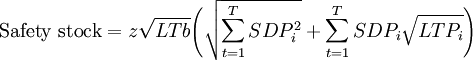
Where:
- LTb = Production lead time for base product
- LTPi = Production lead time for product i (in this case LTb + LTPi must be contrained to 21)
- SDPi = Standard deviation in demand for product i
We may then evaluate the change in safety stock for alternative base product production lead times. As seen in Table 3, only when the base product production lead time equals 19 and 20 days does the level of safety stock decline (by 1% and 8% resepctively). The relationship between base product production lead time and change in safety stock is shown in Chart 1. For all other base product production lead times, safety stock inventory increases relative to the case of no risk pooling (or complete form speculation as shown in Table 1). In these instances, the firm should consider a make-to-stock orientation.
| Table 3: Percentage change (+/-) in Safety Stock at Various Base Product Production Lead Times; In-stock probability = 98% (z=2.05) | |||||||||||||||||||||
|---|---|---|---|---|---|---|---|---|---|---|---|---|---|---|---|---|---|---|---|---|---|
| Base product production lead time (days) | 1 | 2 | 3 | 4 | 5 | 6 | 7 | 8 | 9 | 10 | 11 | 12 | 13 | 14 | 15 | 16 | 17 | 18 | 19 | 20 | |
| Percentage change (+/-) in safety stock | 13% | 17% | 20% | 21% | 22% | 23% | 23% | 23% | 22% | 22% | 21% | 20% | 18% | 16% | 14% | 11% | 8% | 4% | -1% | -8% | |
Example: Risk Pooling Across Space - The Square Root Rule
Risk pooling across space suggests that the objects being aggregated are geographic regions. This is equivalent to geographic postponement since the firm delays descions on where products are needed until after orders have arrived. The primary operationalization of risk pooling across space is through the use of fewer warehouses. Similar to the case of risk pooling across products, the extent of risk reduction will depend on the covariation of demand (positive, negative, null) among the regions. The general experience of the business community is that risk pooling across space associates with lower variance in demand. This ultimately leads to lower safety stock inventory. A heuristic that captures the reduction in demand from risk pooling across space is known as the square root rule[3].
Square Root Rule

Where:
- If = Total inventory at future facilities
- nc = number of current facilities
- nf = number of future facilities
If a business operates five warehouses and the value of inventory at each warehouse equals €100,000, then the total value of inventory equals 5 × €100,000 = €500,000. How much inventory would be needed if one warehouse were operated?
- Given: Ic = €500,000; nc = 5; nf = 1

- Therefore, If = €223,607
- This represents a 55% reduction in inventory
The reduction in invetory from risk pooling across space was obtained through a decline in safety stock. The economic argument for a reduction in the number of warehouses requires a total cost analysis as the use of fewer warehouses may lead to a shift in the underlying transportation cost structrure. Furthermore, the square root rule is a simplified model that assumes: (1) transshipments between facilities is not common; (2) lead times variance is neglible; (3) the service levels across facilities is constant; and (4) the distribution of demand at the facilities is normal.
References
- ↑ Carlton, D.W. (1979), “Vertical Integration in Competitive Markets under Uncertainty,” Journal of Industrial Economics, 27 (3), p.204.
- ↑ Simchi-Levi, D., P. Kaminsky and E. Simchi-Levi (2000), Designing and Managing the Supply Chain, Irwin Mc-Graw Hill, Boston, p.56-60.
- ↑ Zinn, W; M. Levy, and D.J. Bowersox (1989), "Measuring the Effect of Inventory Centralization/Decentralization on Aggregate Safety Stock: The "Square Root Law" Revisited", Journal of Business Logistics, 10 (1), 1-14.


