Полная стоимость владения
Материал из Supply Chain Management Encyclopedia
English: Total cost of ownership
Полная стоимость владения (total cost of ownership, TCO) представляет собой универсальный термин, который обозначает совокупные затраты, с которыми связано использования продукта или услуги на протяжении всего их жизненного срока. В настоящее время термин TCO применяется к целому ряду продуктов и услуг, включая автомобили, заводы, информационные технологии и финансовые услуги. [1] В управлении цепями поставок данный термин часто используется при анализе изменений: например, в проблеме смены поставщиков. При анализе TCO необходимо выделить релевантные виды затрат и обосновать их включение в анализ. Факторы, которые не включаются в анализ TCO, является одинаковыми для всех рассматриваемых альтернатив. Данное предположение, однако, родилось не из практического опыта. Например, довольно трудно измерить гибкость и жизнеспособность альтернативных поставщиков. Ниже мы приводим пример применения анализа TCO в управлении цепями поставок и иллюстрируем сильные и слабые стороны данного подхода.
Пример
Предположим, что XInc является производителем транспортных средств и управляет несколькими сборочными предприятиями.
- Одни стандартный компонент (деталь 125) используется во всех продуктах. Еженедельный спрос на эту деталь составляет 8500 единиц при стандартном отклонении 500. Большой объем спроса объясняется тем, что каждый продукт компании содержат несколько единиц детали 125.
- Некоторое ограниченное количество деталей 125 оказывается дефектными после получения. Половина дефектных частей используется в производстве готового продукта, в результате чего средние затраты на гарантийный ремонт составляются 1000 долл. XInc довольно требовательно относится в проблеме безопасности, связанной с любыми деталями продукта, однако инженеры убедительно продемонстрировали, что в случае дефектности детали 125 безопасность готового продукта никак не страдает. Другая половина дефектных деталей выявляется в течение производственного процесса, при этом затраты на замену и утилизацию неисправной детали составляют 1,05 долл. на единицу.
- Ежегодные затраты на поддержание запасов детали 125 составляет 0,20 долл.;
- XInc необходим высокий уровень доступности комплектующих (???) 99,9%
- От альтернативного поставщика было получено новое предложение и XInc решила использовать анализ TCO для его оценки;
Для текущего поставщика:
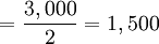
- Установил цены 2.00 доллара за единицу и продает упаковки по 3000 шт.;
- Уровень брака для детали 125 составляет 1/10000;
- XInc, through a supplier evaluation program, has ascertained that the lead time of the current supplier is 10 days, with a standard deviation of 2 days
The potential supplier is offering:
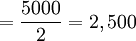
- A selling price $1.93 per unit with a minimum lot size quantities of 5,000
- A lead time of 20 days with a standard deviation of 6 days
- A defect rate of one in 6,000
Which supplier should XInc select?
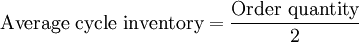
From the data provided, we can evaluate for each supplier the average amount of inventory and the subsequent annual inventory carrying cost, the annual cost of purchased goods, and the annual cost of defects. The first step is to identify the terms required for the analysis and ensure that the time period units are consistent. Since demand (D) is given on a weekly basis, we need to convert the lead time (LT) and its respective variance (σLT), given in days, to reflect weekly time units. As seen in Table 1, lead time (LT), the standard deviation in lead time (σLT), product value (v), and defect rate differ across the current and potential suppliers. Demand (D), the standard deviation in demand (σD), the carrying cost rate (c), and the z value relecting the inventory service level are identical across the two suppliers. Table 2 demonstrates how the average cycle inventory, safety stock, and inventory carrying cost for the expected inventory level were evaluated. The evaluation of safety stock was undertaken using the model provided in inventory model with uncertainty in demand and lead time. Next, the cost of purchased materials is the product of annual demand and the purchase price per unit. Finally the warranty cost is evaluated as the number of defects that are used in finished products multiplied by the $1,000 warranty cost plus the number of units detected within the plants mutiplied by the rehandling, rework, and scrap cost of $1.05. The annual total cost of the current and potential suppliers are $917,221 and $901,052, respectively. The TCO analysis shows that the potential vendor offers a savings of $16,169 over the current vendor.
The TCO assumes that any factors not in the analysis are constant across alternatives.
- Inbound transportation cost, terms of payment, supplier relational capabilities, ordering systems (including EDI and other electronic capabilities) were assumed to be equal across alternatives. Some of these factors (e.g., transportation cost) could be addressed without great difficulty. However, it is difficult to quantify other factors such as relational capabilities for inclusion in a TOC analysis. This is where supplier evaluation and supplier development becomes important additions that supplement the TCO approach
- Another important factor not accounted for in the TCO analysis is the impact of the final product defect rate on revenue. In this specific example, no information was provided on the issue. However, if XInc repeatedly opts for the low cost solution across multiple vendors, then the market might notice the decline in overall product quality. Revenue might then suffer
- The final decision as to the selection of which supplier should provide product part 125 resides in the trade-off that XInc is willing to make between cost and quality. The decision should thus be based on the strategic orientation of XInc (e.g., low cost leader; quality) and the ultimate position that the firm would like to occupy in the marketplace.
| Table 1: Variables in the TCO Analysis | ||
|---|---|---|
| Current Supplier | Potential Supplier | |
| Weekly demand (D) | 8,500 | 8,500 |
| Standard deviation in demand (σD) | 500 | 500 |
| Lead time (LT) | 10/7 = 1.43 | 20/7 = 2.86 |
| Standard deviation in lead time (σL) | 2/7 = .29 | 6/7 = .86 |
| Carrying cost rate (c) | .20 | .20 |
| Replacement value (v) | 2.00 | 1.93 |
| Defect rate | 1/10000 = .0001 | 1/6000 = .000167 |
| A 99.9% inventory service level translation | z = 3.08 | z =3.08 |
| Table 2: Evaluating the Total Cost of Ownership | ||
|---|---|---|

| 
| |
| 
| 
|

| 
| 
|

| 
| 
|

| 
| 
|

| 
| 
|

| 
| 
|


